DTCWT in Pytorch Wavelets
Pytorch wavelets is a port of dtcwt_slim, which was my first attempt at doing the DTCWT quickly on a GPU. It has since been cleaned up to run for pytorch and do the quickest forward and inverse transforms I can make, as well as being able to pass gradients through the inputs.
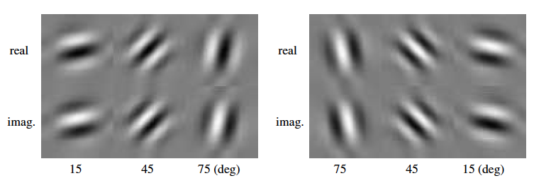
For those unfamiliar with the DTCWT, it is a shift invariant wavelet transform that comes with limited redundancy. Compared to the undecimated wavelet transform, which has \(2^J\) redundancy, the DTCWT only has \(2^d\) redundancy (where d is the number of input dimensions - i.e. 4:1 redundancy for image transforms). Instead of producing 3 output subbands like the DWT, it produces 6, which roughly represent 15, 45, 75, 105, 135 and 165 degree wavelets. On top of this, the 6 subbands have real and imaginary outputs which are in quadrature with each other (similar to windowed sine and cosine functions, or the gabor wavelet).
It is possible to calculate similar transforms (such as the morlet or gabor) using fourier transforms, but the DTCWT is faster as it uses separable convolutions.
Notes
Because of the above mentioned properties of the DTCWT, the output is slightly different to the DWT. As mentioned, it is 4:1 redundant in 2D, so we expect 4 times as many coefficients as from the decimated wavelet transform. These extra coefficients come from:
- 6 subband outputs instead of 3 with ial and imaginary coefficients instead of just real. For an \(N \times N\) image, the first level bandpass has \(3N^2\) instead of \(3N^2/4\) coefficients.
- The lowpass is always at double the resolution of what you’d expect it to be for the level in the wavelet tree. I.e. for a 1 level transform, the lowapss output is still \(N\times N\). For a two level transform, it is \(N/2 \times N/2\) and so on.
Example
import torch
from pytorch_wavelets import DTCWTForward, DTCWTInverse
xfm = DTCWTForward(J=3, biort='near_sym_b', qshift='qshift_b')
X = torch.randn(10,5,64,64)
Yl, Yh = xfm(X)
print(Yl.shape)
>>> torch.Size([10, 5, 16, 16])
print(Yh[0].shape)
>>> torch.Size([10, 5, 6, 32, 32, 2])
print(Yh[1].shape)
>>> torch.Size([10, 5, 6, 16, 16, 2])
print(Yh[2].shape)
>>> torch.Size([10, 5, 6, 8, 8, 2])
ifm = DTCWTInverse(biort='near_sym_b', qshift='qshift_b')
Y = ifm((Yl, Yh))
Like with the DWT, Yh returned is a tuple. There are 2 extra dimensions - the
first comes between the channel dimension of the input and the row dimension.
This is the 6 orientations of the DTCWT. The second is the final dimension, which is the
real an imaginary parts (complex numbers are not native to pytorch). I.e. to
access the real part of the 45 degree wavelet for the first subband, you would
use Yh[0][:,:,1,:,:,0], and the imaginary part of the 165 degree wavelet
would be Yh[0][:,:,5,:,:,1].
The above images were created by doing a forward transform with an input of zeros (creates a pyramid with the correct size bands), and then setting the centre spatial value to 1 for each of the orientations at the third scale. I.e.:
import numpy as np
import torch
from pytorch_wavelets import DTCWTForward, DTCWTInverse
xfm = DTCWTForward(J=3)
ifm = DTCWTInverse()
x = torch.zeros(1,1,64,64)
# Create 12 outputs, one for the real and imaginary point spread functions
# for each of the 6 orientations
out = np.zeros((12,64,64)
yl, yh = xfm(x)
for b in range(6):
  for ri in range(2):
    yh[2][0,0,b,4,4,ri] = 1
    out[b*2 + ri] = ifm((yl, yh))
    yh[2][0,0,b,4,4,ri] = 0
# Can now plot the output
Advanced Options
There is a whole host of advanced options for calculating the DTCWT. The above example shows the use case that will work most of the time. However, here are some more ways the DTCWT can be done:
Custom Biorthogonal and Qshift Filters
Rather than specifying the type of filter for the layer 1 (biort), and layer 2+ (qshift) transforms, you can provide the filters directly. They should be given as a tuple of array-like objects. For the biorthogonal filters, this is a 2-tuple of low and highpass filters. For the qshift filters, this will be a 4-tuple of low for tree a, low for tree b, high for tree a and high for tree b filters.
E.g.:
from pytorch_wavelets import DTCWTForward
from pytorch_wavelets.dtcwt.coeffs import biort
# The standard style
xfm1 = DTCWTForward(biort='near_sym_a', J=1)
# Get our own filters, here we reverse the standard filters so they
# still have the right properties, only changing the phase
h0o, _, h1o, _ = biort('near_sym_a')
xfm2 = DTCWTForward(biort=(h0o[::-1], h1o[::-1]), J=1)
Note that you must be careful when doing this, as the filters are designed to have the correct phase properties, so any changes will likely result in a loss of the quarter shift and hence the shift invariant properties of the transform.
Skipping Highpasses
There is the option to not calculate the bandpass outputs at given scales. This can speed up the transform if you know that there is very little useful content in some areas of the frequency space. To do this, you can give a list of booleans to the skip_hps parameter (if it is a single boolean, that is then used for all the scales). The first value corresponds to the first scale highpass outputs, and a value of true means do not calculate them.
E.g.:
from pytorch_wavelets import DTCWTForward
xfm = DTCWTForward(J=3, skip_hps=[True, False, False])
yl, yh = xfm(torch.randn(1, 1, 64, 64))
print(yh[0].shape)
>>> torch.Size([0])
print(yh[1].shape)
>>> torch.Size([1, 1, 6, 16, 16, 2])
Naturally, the inverse transform happily accepts tensors with 0 shape (or even None’s) and sets that level to be all zeros.
Changing the output shape
By default the highpass outputs have an extra 2 dimensions, one at the end for complex values, and one after the channel dimension, for the 6 orientations. E.g. an input of shape of \((N, C_{in}, H_{in}, W_{in})\) will have bandpass coefficients with shapes \(list(N, C_{in}, 6, H_{in}'', W_{in}'', 2)\), (we’ve put dashes next to the height and width as they will change with scale).
You can choose where the orientations and real and imaginary dimensions go with the options o_dim and ri_dim, which are by default 2 and -1.
Including all the lowpasses
In case you want to get all the intermediate lowpasses, you can with the include_scale parameter. This works a bit like the skip_hps where you can provide a single boolean to apply it to all the scales, or a list of booleans to fine tune which lowpasses you want.
If any of the value in include_scale is true, then the transform output will change, and the lowpass will be a tuple.
E.g.
from pytorch_wavelets import DTCWTForward
xfm1 = DTCWTForward(J=3)
xfm2 = DTCWTForward(J=3, include_scale=True)
xfm3 = DTCWTForward(J=3, include_scale=[False, True, True])
x = torch.randn(1, 1, 64, 64)
yl, yh = xfm1(x)
print(yl.shape)
>>> torch.Size([1, 1, 16, 16])
# Now do xfm2 which will give back all scales
yl, yh = xfm2(x)
for l in yl:
  print(yl.shape)
>>> torch.Size([1, 1, 64, 64])
>>> torch.Size([1, 1, 32, 32])
>>> torch.Size([1, 1, 16, 16])
# Now do xfm3 which will give back the last two scales
yl, yh = xfm3(x)
for l in yl:
  print(yl.shape)
>>> torch.Size([0])
>>> torch.Size([1, 1, 32, 32])
>>> torch.Size([1, 1, 16, 16])
Note that to do the inverse transform, you have to give the final lowpass output. You can provide None to indicate it’s all zeros, but you cannot provide all the intermediate lowpasses.